Research
How the search works
This page is the methodology, written to be argued with. If a step here does not hold up, the predictions built on it do not either.
What Chestly claims. It identifies candidate locations worth investigating on the ground. It does not claim that satellite imagery alone confirms a tree’s species.
Results at a glance
How well the model actually performs
Every figure below is out-of-fold: scored by a model that never saw that site or its 25 km spatial block. These are the numbers the release gate reads.
ROC-AUC
0.774
Separates chestnut sites from non-chestnut sites on unseen ground
0.5 = chance · 1.0 = perfect
PR-AUC
0.538
Ranking quality when positives are rare
vs a base rate of 0.24
Precision@100
83%
Share of the top 100 ranked sites that were real chestnut sites
retrospective, on held-out geography
Brier
0.159
Gap between stated probabilities and reality
lower is better
Reading Precision@100: it describes how the ranking behaved on held-out geography during validation. It does not mean a published candidate has that percentage probability of containing a chestnut — no number on this site means that.
Where the search is open — and where it is not
Each state faces the same fixed gate before a single candidate is published there: ranking accuracy, lift over the base rate, top-of-ranking precision, and calibration. A state that fails stays failed, and the reason is published.
PAPennsylvania
LiveHome region of the deployed model; spatially validated and searched statewide.
24 candidatesVAVirginia
LivePassed the transfer validation gate; searched statewide.
25 candidatesTransfer ROC-AUC 0.805WVWest Virginia
GatedThe Pennsylvania model does not yet meet the deployment gate here (probability calibration failed on held-out sites). No candidates are published for this state.
No candidates publishedTransfer ROC-AUC 0.768MDMaryland
GatedThe Pennsylvania model does not yet meet the deployment gate here (probability calibration failed on held-out sites). No candidates are published for this state.
No candidates publishedTransfer ROC-AUC 0.779NYNew York
GatedThe Pennsylvania model does not yet meet the deployment gate here (ranking accuracy below the deployment gate; too little lift over the base rate; top-of-ranking precision below the gate; probability calibration failed on held-out sites). No candidates are published for this state.
No candidates publishedTransfer ROC-AUC 0.662OHOhio
GatedThe Pennsylvania model does not yet meet the deployment gate here (ranking accuracy below the deployment gate; too little lift over the base rate; probability calibration failed on held-out sites). No candidates are published for this state.
No candidates publishedTransfer ROC-AUC 0.671
What did not work
Null and negative results are kept in full below, at the same prominence as the positive ones.
Flowering detection failed
Sentinel-2 cannot detect chestnut flowering at 10 m. The channel was retired rather than reported as a partial success.
Four states are gated
The model does not meet its deployment gate in WV, MD, NY or OH, so it publishes nothing there.
Top-25 lists do not rediscover known trees
In a held-out backtest, no model recovered known trees at candidate-release depth. Enrichment shows up shallower in the ranking.
Two model upgrades were rejected
A six-state retrain and an ecoregion-adaptive architecture both failed pre-registered acceptance criteria and were not deployed.
The rest of this page is the full methodology, in order, from the observations through to field validation.
The question
Chestly does not ask 'is this pixel an American chestnut?' No satellite currently in orbit can answer that. Sentinel-2 resolves the ground at 10 metres; a single mature tree's canopy is often smaller than one pixel and is always mixed with its neighbours.
The question it does ask is: given everything known about where surviving American chestnuts have been documented, which patches of forest most resemble those places, and which of those are worth a person's time to visit?
That reframing matters. It turns an identification problem, which is currently unsolvable from imagery, into a search-prioritisation problem, which is not.
The pipeline, in pictures
Thirteen figures, generated directly from the current pipeline's data — regenerated whenever the pipeline runs, never drawn from memory. Panels that use a chosen best-case example say so in their caption; the validation panel is computed only on spatially held-out predictions and is kept deliberately separate from the illustrations.
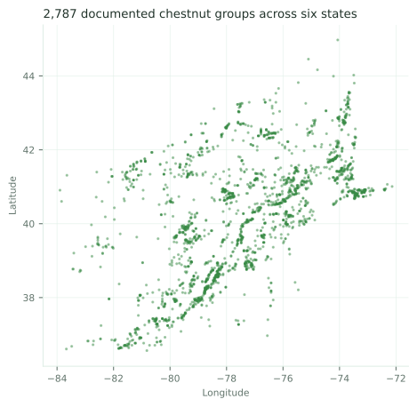
01 Documented observations
The data: Every wild, precisely-located American chestnut observation group used in training, from iNaturalist, across PA, WV, VA, MD, NY and OH.
What Chestly looks for: Where the species demonstrably survives today.
Why it matters: These points are the only ground truth the search has; everything downstream is an extrapolation from them.
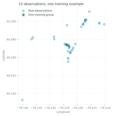
02 Grouping repeat observations
The data: A well-documented stand (chosen for clarity): every raw record within ~2 km against the single group the model trains on.
What Chestly looks for: Repeat records of the same tree, which would otherwise be counted as many independent examples.
Why it matters: Without grouping, popular trees dominate training and validation leaks -- the model would be graded on trees it already memorised.
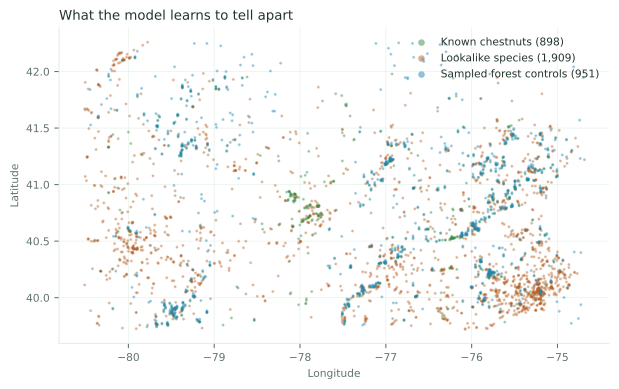
03 Tiered negative data
The data: Pennsylvania training sites: known chestnuts, community-confirmed lookalike species, and habitat-matched plus randomly sampled forest controls.
What Chestly looks for: The discriminations that matter: chestnut vs Chinese chestnut, chestnut oak and beech, and chestnut forest vs ordinary forest.
Why it matters: A model trained against randomly sampled forest alone learns 'places people go'; the tiers force it to learn the species instead.
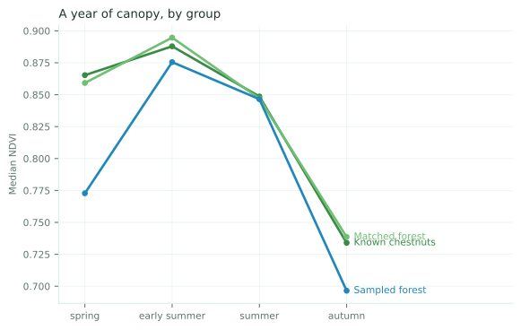
04 Seasonal phenology
The data: Median seasonal NDVI trajectories for chestnut sites, habitat-matched forest and randomly sampled forest, from cloud-masked Sentinel-2 composites.
What Chestly looks for: Timing differences -- when a canopy greens up and senesces -- not just how green it is in August.
Why it matters: Phenology is among the few signals that can separate species that look identical in a single image.
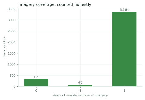
05 Coverage honesty
The data: How many usable (cloud-masked) years of satellite imagery each training site actually has.
What Chestly looks for: Sites where cloud masking left too little imagery -- recorded as missing rather than imputed into a fake signal.
Why it matters: Absence of evidence is stored as absence; a model fed silently filled-in seasons learns the filler.
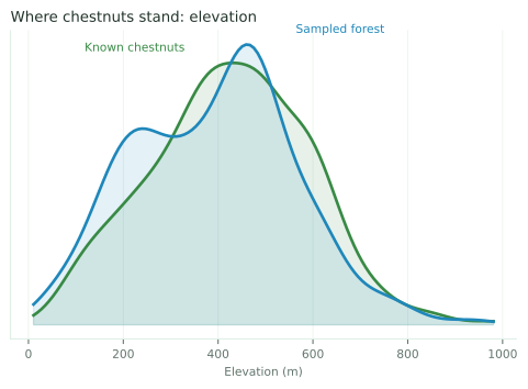
06 Where chestnuts stand: elevation
The data: Elevation distributions of known chestnut sites against randomly sampled forest controls (Copernicus GLO-30 terrain).
What Chestly looks for: The mid-elevation ridge-and-slope band the species survives on.
Why it matters: Terrain is the strongest single predictor the model has -- and it is visible to anyone, which keeps the model auditable.
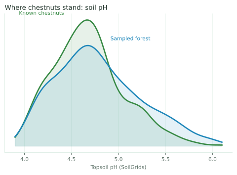
07 Where chestnuts stand: soil pH
The data: Topsoil pH distributions of known chestnut sites against randomly sampled forest controls.
What Chestly looks for: The acid end of the scale: chestnuts hold to well-drained, acidic soils.
Why it matters: Soil chemistry is why the model transfers along the Appalachians and fails toward calcareous Ohio -- the domain-shift report made that measurable.
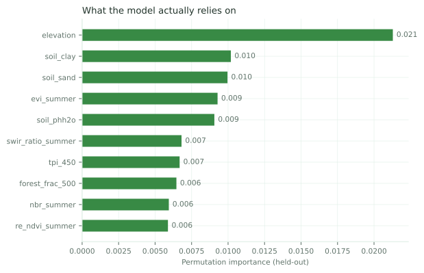
08 Feature importance
The data: Top-10 permutation importances of the deployed model, measured on spatially held-out data.
What Chestly looks for: Whether the learned reliance matches chestnut ecology: elevation, soil acidity and texture, topographic position, red-edge spectra.
Why it matters: A model relying on sensible biology transfers; one relying on artefacts collapses off its home turf. This is checkable here.
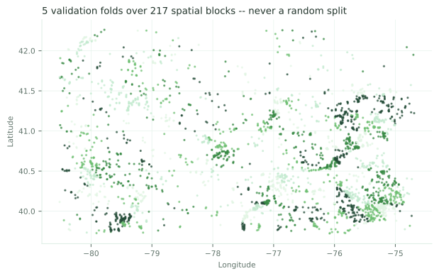
09 Spatial validation
The data: Every training site shaded by its cross-validation fold; folds are built from ~25 km blocks (217 of them), so neighbouring sites are never split across train and test.
What Chestly looks for: Whether the model can score geography it has never seen -- the only question that predicts field performance.
Why it matters: A random split would grade the model on near-copies of its training data and overstate everything.
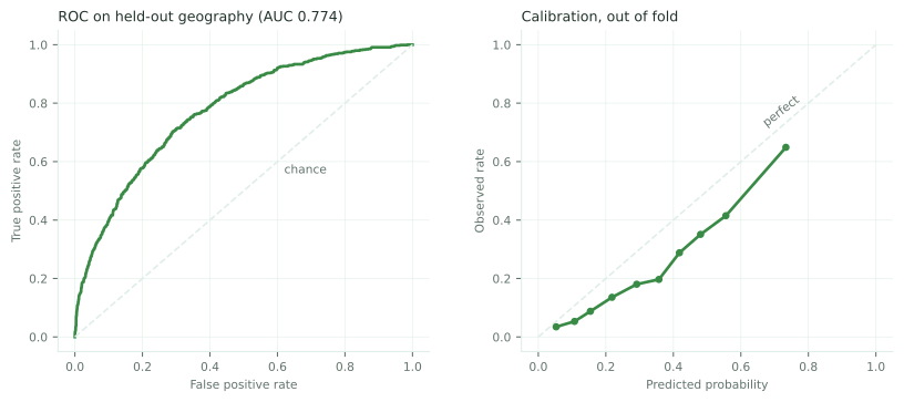
10 The gate, measured
The data: Unbiased validation of the deployed model: ROC and calibration, computed only from predictions on sites in held-out spatial folds.
What Chestly looks for: Whether the model clears the fixed release gate -- and whether a stated 70% behaves like 70%.
Why it matters: These are the numbers the release gate reads. They are never mixed with the illustrative panels around them.
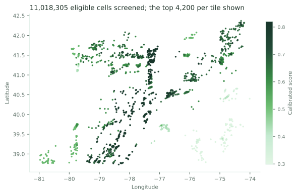
11 Statewide screening
The data: Stage-1 screening of Pennsylvania: every eligible 120 m forest cell scored, with the strongest cells per satellite tile plotted.
What Chestly looks for: Where model support concentrates at state scale -- the raw material for the map's heatmap.
Why it matters: Screening at 120 m makes a statewide search affordable; everything that survives is re-measured exactly before release.
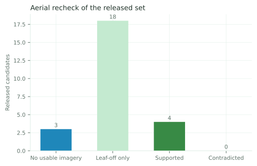
12 High-resolution recheck
The data: NAIP 0.6 m aerial outcomes for the released candidates: supported, contradicted (down-ranked), leaf-off only, or no probative imagery.
What Chestly looks for: Open ground, buildings or bare fields hiding inside a 120 m 'forest' cell -- and crowns consistent with a canopy chestnut.
Why it matters: Missing imagery is reported as missing, never as a low score; only leaf-on imagery is allowed to contradict a candidate.
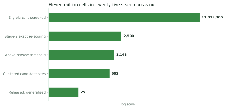
13 From state to shortlist
The data: The Pennsylvania release funnel: screened cells, exact re-scoring, the fixed score threshold, clustering, and the released set (bar length is log-scaled; the printed counts are exact).
What Chestly looks for: Ruthless narrowing, with each cut made by a rule fixed in advance.
Why it matters: A shortlist a person can actually field-check is the product; the funnel is what makes 25 defensible.
Where the observations come from
Documented American chestnut observations are sourced from iNaturalist, retrieved through its public API and refreshed by an ingestion step that updates existing records rather than duplicating them. Each record on the map links back to the original.
These are community-contributed records. They carry two kinds of uncertainty that matter here: whether the identification is correct, and how precisely the location was recorded. Both are stored alongside the observation and shown on the map rather than smoothed away.
iNaturalist assigns each record a quality grade. Research Grade means enough independent identifiers have agreed — a useful filter, and the map's default, but a community consensus rather than a determination. American chestnut is regularly confused with Chinese chestnut and chestnut oak, so a Research Grade record is strong evidence and not proof.
Where iNaturalist obscures a record's coordinates, that decision is respected. Obscured records publish a deliberately imprecise point, are flagged as such in the interface, and no attempt is made to recover the true location. Cultivated and planted trees are excluded by default: a chestnut somebody planted says nothing about where a wild survivor might stand.
Training data
Positive examples come from documented observations of Castanea dentata, primarily iNaturalist records, filtered for identification quality and positional accuracy. Cultivated and planted trees are excluded where they can be identified: a chestnut somebody planted says nothing about where a wild survivor might stand.
Every observation carries a confidence value rather than being treated as ground truth. Community identifications are evidence and are sometimes wrong, particularly against Chinese chestnut and chestnut oak.
Where a source obscures a record's location for conservation reasons, that designation is preserved. An obscured point is a random position inside a large box, and treating it as precise would sample satellite features from the wrong forest entirely.
Negative data
Comparing chestnut observations against randomly chosen forest would produce a model that separates 'places people go' from 'places people do not go'. The negative set is built deliberately instead.
Hard negatives are confirmed observations of species that look or behave similarly: Chinese chestnut, chestnut oak, American beech, and selected oaks and maples. These are the discriminations that actually matter, and they are the ones a naive negative set never teaches.
Geographic negatives are forest near known chestnut habitat with nothing on record. They are stored with low confidence and down-weighted during training, because absence of an observation is not absence of a tree. Treating them as confident negatives would teach the model that undocumented chestnuts are non-chestnuts — precisely backwards for a project trying to find undocumented chestnuts.
Satellite data
Sentinel-2 L2A surface reflectance, discovered through the public Earth Search STAC catalogue and read directly from the open-access archive on AWS. Only the pixels around each study site are fetched — windowed reads from cloud-optimised GeoTIFFs — so no whole scenes are downloaded or stored.
Every scene is masked with its scene-classification layer before use: cloud, shadow, cirrus and defective pixels are discarded, and each seasonal window is reduced to a median composite of what remains. Where masking leaves too little clear imagery, the window is marked missing rather than filled in.
From each composite the pipeline computes vegetation indices and band ratios, and retains the underlying bands — including the red-edge bands, which sit on the steep reflectance transition between red and near-infrared and are among the few places Sentinel-2 can plausibly separate species that look alike in visible light.
Phenology
Phenology — the timing of a canopy's annual cycle — is likely the strongest available signal. Two species can reflect almost identically in August and still leaf out three weeks apart.
Four windows are composited each year: spring leaf-out, the early-summer flowering period, peak summer canopy, and autumn senescence. American chestnut flowers conspicuously in early summer, with creamy-white catkins covering the crown, and that window carries the most distinctive expected signature — an expectation Chestly has now tested directly, with results reported honestly in the flowering experiment section below.
Window dates are configured per region and shifted with latitude, because spring arrives roughly three days later per degree northward in the eastern United States. A fixed calendar window would compare leaf-out in one place to full canopy in another and call the difference a species signal.
The flowering experiment
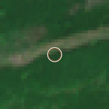
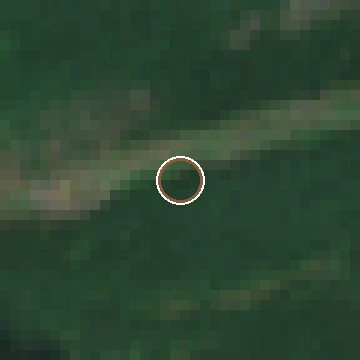
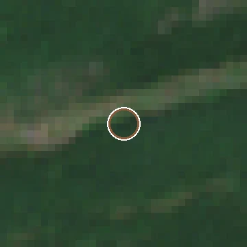
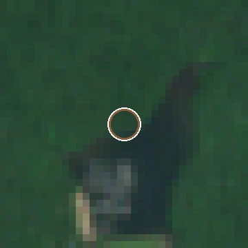
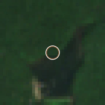
The flowering hypothesis was attractive enough to deserve a real test rather than an assumption. In summer 2026 Chestly ran one: can Sentinel-2 detect American chestnut flowering strongly enough to help identify trees? The design used every Pennsylvania iNaturalist record with a community flowering annotation, habitat-matched forest controls a few hundred metres from each tree, Chinese chestnut records as a specificity control, and five years of imagery per site — with features measuring both change over time and contrast against the immediately surrounding canopy.
The honest answer is no — not at this resolution, with this method. Individual seasonal changes at chestnut sites are real and measurable, but they do not separate chestnuts from ordinary forest: the flowering-window brightening the hypothesis predicts shows up no more often at confirmed flowering chestnuts than at their paired controls, and nothing tested distinguishes American chestnut from Chinese chestnut. Adding flowering features to a baseline habitat model made spatially held-out classification slightly worse, not better.
The failure modes were instructive. The largest apparent flowering-window brightening in the whole dataset traced to thin cirrus haze that the standard cloud mask passes — an artefact that would have looked like a discovery under a less suspicious analysis. And the strongest 'signal' found — chestnut sites differing from surrounding canopy — is static across seasons, which means it reflects where these trees grow, not the flowering event.
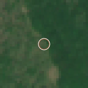
A null result changes the architecture, not the mission. Flowering evidence is retired as an identification signal at 10 m; habitat and general phenology carry the model until higher-resolution imagery or a better method reopens the question. The figures below show the experiment's raw material at its most favourable: three confirmed flowering chestnuts, chosen deliberately as the strongest measured cases with verified-clear imagery. Even here, the flowering window looks like forest.
Before flowering
2024-05-24
Flowering window
2024-07-13
After flowering
2024-07-28
Before flowering
2023-05-30
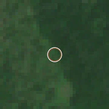
Flowering window
2023-07-14
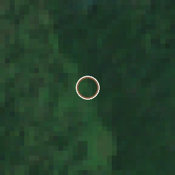
After flowering
2023-08-01
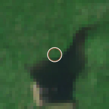
Before flowering
2021-05-20
Flowering window
2021-06-29
After flowering
2021-08-13
Habitat modelling
Imagery is not the only input. A separate habitat score is built from elevation, slope, aspect, forest cover and structure, distance from development, and soil characteristics where they are available.
Aspect is decomposed into northness and eastness before it reaches a model. Raw aspect in degrees is circular: 1 and 359 describe adjacent slopes but sit at opposite ends of the numeric range, which a tree-based model would happily split on.
An eligibility mask runs before anything is scored, removing water, dense development, highways, large agriculture and terrain outside the elevation and slope ranges the species tolerates. This is both a correctness measure and what makes state-scale inference affordable.
Machine learning
Three models compete on identical spatially blocked folds: logistic regression, a Random Forest, and gradient boosting (LightGBM). Not a neural network: with hundreds rather than millions of positive examples, a deep model would mostly memorise them, and there is no way to tell that apart from success without honest validation first.
The Random Forest won on held-out geography and calibration, and the simpler logistic baseline was close enough to confirm the signal is real rather than an artefact of model capacity. Selection preferred the simplest model within a hair of the best score.
The output is a probability that a location is worth investigating. It is not a probability that a chestnut is present, and the site does not present it as one.
The general model, measured
The first gated release of the general model was trained on 898 grouped chestnut sites — every Research Grade, precisely located, wild Pennsylvania record, with repeat observations of the same tree collapsed into one — against 2,860 tiered negatives: community-confirmed lookalike species, habitat-matched forest a few hundred metres from each chestnut, and randomly sampled forest as the weakest tier.
Every number below is out-of-fold from spatial cross-validation: scored by a model that never saw that site or its 25 km block. Before any statewide inference was allowed, the model had to clear a five-part gate fixed in code in advance — materially above chance on spatial holdouts, ranking precision double the base rate, no regional collapse, and probabilities that beat the base-rate predictor. It cleared all five.
The figures that follow separate two kinds of content deliberately: the metrics table is unbiased validation; the comparison table, seasonal profile and aerial pairs are explanatory illustrations, chosen to be clear rather than average.
What a released candidate looks like: the top-ranked site in the first experimental set is a forest cell on an upper slope in eastern Pennsylvania, 6.8 km from the nearest documented chestnut, scored 0.82 by the general model with habitat and phenology channels agreeing, and its flowering-window 2022 aerial imagery was independently consistent with known chestnut crowns (a weak signal, weighted accordingly). What rejection looks like: three otherwise high-scoring clusters were down-ranked because their leaf-on aerial imagery showed open ground where coarser layers saw forest — the refinement stage doing exactly its job.
Held-out performance (spatial blocks the model never saw)
ROC-AUC
0.774
0.5 = chance
PR-AUC
0.538
base rate 0.24
Precision@100
83%
top of the ranking
Brier
0.159
lower is better
898 grouped chestnut sites vs 2860 tiered negatives across 217 ~25 km spatial blocks. Held-out regions stay stable: west 0.79, central 0.76, east 0.74.
What a chestnut site looks like, in numbers
| Median value | Known chestnuts | Matched forest | Randomly sampled forest |
|---|---|---|---|
| Elevation (m) | 428.765 | 406.091 | 422.396 |
| Soil pH | 4.7 | 4.7 | 5 |
| Sand (%) | 37.6 | 36.3 | 30 |
| Forest within 500 m | 0.982 | 0.976 | 0.882 |
| Topographic position (m) | 5.208 | -0.448 | -1.262 |
| Slope (deg) | 7.154 | 7.877 | 6.887 |
| Canopy height (m) | 14.094 | 15.077 | 13.336 |
| Summer NDVI | 0.849 | 0.847 | 0.847 |
The seasonal profile, and why it is not enough alone
What stays hard (held-out AUC vs known chestnuts)
- Habitat-matched forest (500–900 m from a chestnut)0.64
- Nearby forest (1.5–3 km)0.67
- Chestnut oak0.69
- Randomly sampled Pennsylvania forest0.77
- American beech0.82
- Tulip poplar0.85
- Red maple0.86
- Allegheny chinquapin0.87
- Northern red oak0.87
- Chinese chestnut0.93
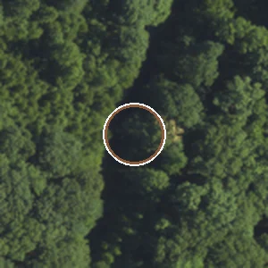
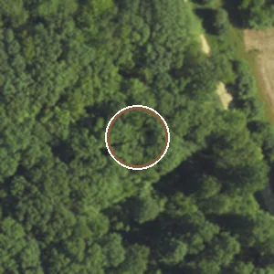
What 0.6 m aerial imagery adds
Confirmed chestnut
iNaturalist #190894349 · 2022-07-03
Matched forest control
~500–900 m away · same date
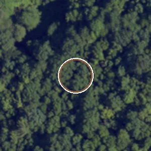
Confirmed chestnut
iNaturalist #89187828 · 2022-06-25
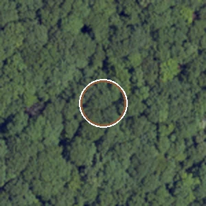
Matched forest control
~500–900 m away · same date
Validation
Splits are geographic, never random. Observations of the same stand share pixels, weather, terrain and often the same photographer; a random split puts near-copies of the training data into the test set, and the model scores beautifully while finding nothing in the field.
Training, validation and test geographies are separated by county or by spatial block. A final holdout geography is not used for training, feature selection or hyperparameter choice, and is scored once at the end. Its entire value is that nothing about the model was chosen with knowledge of it.
Accuracy is not reported as a headline. Against a landscape of forest holding a few hundred known chestnuts, predicting 'none' everywhere scores above 99% accurate and is worthless. What is tracked is precision at the top of the ranking — precision@10, @50, @100 — alongside PR-AUC, Brier score and a calibration curve, because a stated 85% confidence should mean 85%.
Limitations
Sentinel-2 cannot identify an individual tree. A candidate is a patch of forest whose seasonal behaviour resembles places chestnuts are known to survive — nothing stronger.
Training data is biased towards where people walk. Roads, trails and popular parks are over-represented among documented observations, and a model fit to them can learn accessibility as much as habitat. This is a known weakness, not a solved one.
Blighted chestnuts usually persist as understory sprouts beneath a closed canopy, effectively invisible from above. The trees this method can plausibly find are the large, canopy-reaching survivors — which are also the rarest and the most valuable.
Mixed pixels, cloud gaps, terrain shadow and year-to-year weather all inject noise. A signal that does not recur across multiple years should not be trusted, and multi-year stability is a planned filter rather than an implemented one.
The discovery backtest
The question the whole system exists to answer, asked retrospectively: if the trees documented in eastern Pennsylvania were not yet documented, would this pipeline have pointed a volunteer at them? The eastern longitude band — 211 known chestnut groups — was held out entirely, along with anything within 1 km of one of them, and its 839,462 eligible forest cells were re-screened by models that had never seen the band.
At candidate-release depth, no model rediscovered a known tree: zero of 211 recovered in any top-25. A 25-candidate release is a ranked bet on plausible habitat, not a tree detector — which is exactly what this site claims it is, now with a measured number behind the claim.
Deeper in the ranking the models do beat chance: roughly 2× enrichment over a computed random baseline at the top 0.1–0.5%, and the pooled model's top 100 reached 24× the random rate. But at 1% depth both models fell below random. The most plausible reading is the accessibility bias measured from the other side — documented trees sit where people walk, while the model's deep ranking concentrates on remote ridge habitat nobody has surveyed. That is an interpretation offered as such, not an excuse; the numbers stand either way.
Two rejected upgrades
Two attempts to improve the deployed model were built, validated and then rejected against criteria fixed in code before any result was seen. Both rejections are reported here because a project that only publishes its successful experiments is not reporting anything.
A six-state regional retrain (v2.0) improved mean ranking accuracy across the new states, and still failed: Pennsylvania precision@100 fell from 0.83 to 0.72, past the pre-registered 0.05 tolerance. The improvement was real and the cost landed exactly where field planning lives, at the top of the ranking.
An ecoregion-adaptive architecture went further — EPA Level III background baselines built from randomly sampled forest, percentile and deviation forms of soil and terrain variables, latitude-residualized phenology, and per-ecoregion calibration. Contextual features did not improve transfer into unseen states (leave-one-state-out ROC 0.725 with context vs 0.733 without), and every pooled variant repeated the same Pennsylvania regression. Neither was promoted; the deployed model is unchanged.
What survived is the framework rather than a bigger model: a configuration-driven onboarding pipeline that ingests a new state, measures how far its environment has drifted from the training domain, tests transfer, and either unlocks inference or publishes an explanation of the failure.
Field validation
Nothing here is confirmed from a screen. A candidate becomes meaningful only when somebody walks to it and looks, and the metric that matters in the long run is field-confirmed chestnuts divided by field investigations. The workflow below is how a model output becomes — or fails to become — a verified tree.
Approved volunteers claim a candidate before visiting it. A claim reserves the search area, unlocks its exact location for that volunteer only, and expires if unused; it is operational bookkeeping and changes nothing scientific. Candidates on private land stay in the system as scientifically interesting but are not field-trip destinations — nobody is ever pointed onto land they have no right to enter.
A field check is structured observation, not identification. The report asks for photographs — whole tree, leaves, twig and buds, bark, canopy, plus flowers and burs if present — measurements, and simple observations. The visitor is deliberately not asked to decide the species; the photographs carry that burden later, in front of people qualified to judge them.
A report of a possible chestnut moves the candidate to 'possible chestnut — awaiting expert review'. It can never move it to verified: verification is a reviewed decision recorded with its source and date, made by a human examining the evidence, and usually worth an independent confirmation such as an iNaturalist submission or a herbarium sample.
Every outcome feeds the model as a stored label — confirmed chestnuts, confirmed non-chestnuts, and inconclusive visits alike. False positives are the most instructive records in the system and are preserved, never deleted. Nothing retrains automatically: field labels accumulate until a human decides a retraining run is warranted, and any retrained model faces the same spatial-validation gate as its predecessor before it can publish a single candidate.
Confirmed trees are reported to researchers and landowners rather than published. Exact coordinates of unverified candidates and newly confirmed trees are withheld from public maps as a standing rule, not a case-by-case judgement.
1Model
Ranks forest by resemblance to documented chestnut sites. Output: a score, never a species claim.
2Candidate
A generalised public search area. Exact location withheld; land access assessed.
3Field check
A volunteer claims the candidate, walks the area, and records photos and measurements.
4Identification
Experts judge the photographs. The visitor is never required to decide the species.
5Verification
A reviewed decision with source and date. A form submission can never set it.
6Model feedback
The outcome is stored as a label — kept even (especially) when the model was wrong.